The goal of this project is to reproduce the methods and experiments of
the following paper:
C. Cortes, X. Gonzalvo, V. Kuznetsov, M. Mohri, S. Yang AdaNet:
Adaptive Structural Learning of Artificial Neural
Networks. We will try to
reproduce their method that consists in building neural networks whose
structure is learned and optimized at the same time as it’s weights.This
method will be applied to a binary classification task on images from
the CIFAR-10 dataset.
How does Adanet work?
The network’s structure is generated. The full network, which we will call AdaNet, is augmented at each iteration by a sub-network. This sub-network is chosen in regard to it’s effect on an objective function. This allows us to select the best possible sub-network to add to AdaNet at each step. To be able to understand how this process works we will be using the following notation: \(f_t\) the AdaNet network at step \(t\), \(h_t\) and \(h’t\) the candidate sub-networks at step \(t\). For each of these sub-networks, \(h{t,k}\) is the \(k^{th}\) layer and \(h_{t,k,j}\) the \(j^{th}\) neuron in layer \(k\). \(l\) is the maximum number of layers in the sub-network, so \(k\leq l\).
The algorithm, executes the following steps:
-
Network initialization: The input and output layers are generated.
-
Candidate sub-networks generation: 2 candidate sub-networks, \(\mathbf{h}\) and \(\mathbf{h’}\), are generated (cf. figure below):
- One with a depth identical to the sub-network selected in the previous step \(\rightarrow k\)
- One that is deeper by 1 level than the previously selected sub-network \(\rightarrow k+1\)
Both of these sub-networks follow the same connectivity rules. The first layer of the candidate sub-networks \(h_{t,1}\) is connected to the input layer of \(f_t\), the last layer of the candidate sub-networks, \(h_{t,l}\) is connected to the output layer of \(f_t\). For the intermediary layers, each layer \(h_{t,k}\) is connected to the layer below \(h_{t,k-1}\), and can be conncted (randomly) to any of the lower layers of th epreviously selected sub-networks, that is to say \(h_{t\in[1,t-1], k-1}\).
During the first iteration, only the sub-network that augments the depth can be generated since \(k=0\). -
Sub-network choice: From the 2 candidate sub-networks \(\mathbf{h}\) and \(\mathbf{h’}\), we chose the one that minimises the most the following objective function:
$$ \begin{aligned} F_t(\mathbf{w,h}) = \frac{1}{m}\sum^m_{i=1}\Phi(1-y_if_{t-1}(x_i)-y_i\mathbf{w\cdot h}(x_i)) \\ + \mathcal{R}(\mathbf{w,h}) \end{aligned} $$\(x_i\) being the training samples, \(y_i\) their labels, \(m\) the number of training samples, \(\mathbf{w}\) the weights of the candidate sub-network \(\mathbf{h}\) and \(\Phi\) either the exponential or the logistic function. \(\mathcal{R}(\mathbf{w,h})\) is a regularization term left at \(0\) during experimentation.
If \(F(\mathbf{w,h}) > F(\mathbf{w, h’})\), the chosen sub-network is \(\mathbf{h’}\) and \(h_t\leftarrow\mathbf{h’}\). -
Stop condition: Once the best sub-network is selected, we see if it ameliorates AdaNet. If the objective function of the training of \(f_{t-1}\) (which is not the same as the one used to select the best candidate sub-network) is better with the sub-network rather than without, then: \(f_t \leftarrow f_{t-1}+ \mathbf{w^*h}t\). Otherwise \(f{t-1}\) is returned and the algorithm is stopped. If this stop condition is never met, the algorithm stops after \(T\) iterations and returns \(f_T\).
It is easy to see that the generation of the network as well as the weights optimization occurs iteratively at each step of the algorithm.
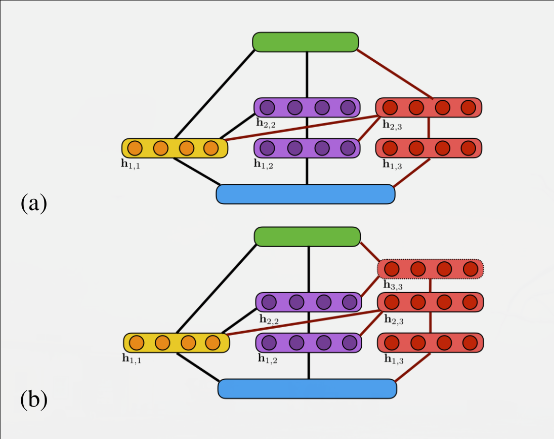 Both of the candidate networks generated at step \(3\) (red), one of
them with a depth of \(2\) (a), like the previously selected sub-network
(blue), and one of depth \(3\) that adds a depth level. Both of these
potential AdaNet networks are the ones that will be evaluated.
Both of the candidate networks generated at step \(3\) (red), one of
them with a depth of \(2\) (a), like the previously selected sub-network
(blue), and one of depth \(3\) that adds a depth level. Both of these
potential AdaNet networks are the ones that will be evaluated.
Experimental choices
Dataset choice
One of two experiments on different datasets had to be chosen:
-
CIFAR-10 dataset
-
Criteo dataset
The choice was made on the size of the respective datasets. If we concentrate on a given binary classification task, CIFAR has \(\approx 10000\) samples per class, whereas the Criteo dataset has \(30\) million. Therefore, considering our limited resources, the choice was made to work on the CIFAR-10 dataset.
API choice
All programs were coded in Python using the Keras API for neural
networks because of it’s simple syntax and high modularity. The
TensorFlow backend is used but it has no influence on the Keras
code.
Ambiguities in the paper
Multiple input tensors management
When a layer, is connected (on the input side), to more than one layer of the other sub-networks, it is unclear if the tensors are:
-
juxtaposed (
concatenatefunction) -
added (
addfunction)
Sub-network regularization
It is not explicitly stated wether the sub-networks are regularized using an \(L_1\) or \(L_2\) norm. The usage of \(\lambda\) term leads us to believe that an \(L_1\) norm was used. It is also unclear wether it is the loss function or the weights during training that are regularized. We have chosen to the weights of each layer of the sub-networks as well as the general output layer with an \(L_1\) norm.
Implementation choices
Input data pre-processing
To be able to use images outside of a Convolutional Neural Network framework, we vectorize the images to a vector of size \(width\cdot height\cdot 3\)
Input and output layers architecture
-
The input layer is of size \(width\cdot height\cdot 3\), which is equal to \(3072\) in the case of CIFAR-10.
-
The output layer is composed of a single neuron with a sigmoid activation function, since the classification task is binary.
Sub-network generation
We chose to generate the sub-networks randomly. Each layer is connected to the preceding layer in it’s own sub-network, however connections to the lower layers in previously selected sub-networks are made randomly.
Objective function
\(x_i\) being the training samples, \(y_i\) their labels, \(m\) the number of
training samples, \(\mathbf{w}\) the weights of the candidate sub-network
\(\mathbf{h}\) and \(\Phi\) the exponential function.
\(\mathcal{R}(\mathbf{w,h})\) is a regularization term left at \(0\) during
experimentation.
We interpret the formula as the following one:
Practical implementation
We have tried to be as faithful as possible with regard to the implementation in the paper. We had to make some decisions however, when the paper did not explicitly state what method was used.
Generation and selection of sub-networks
We give the algorithm a reps parameter, allowing us to specify how many candidate sub-networks are generated at each iteration. Seeing as there are only 2 types of sub-networks generated (equal depth or depth + 1), we have chosen to generate same-depth sub-networks for the \(\frac{reps}{2}\) first-generation steps, and deeper sub-networks for the remaining generation steps.
Connections between the different layers follow the connectivity rules laid out earlier, that is to say: the last layer of the sub-network is connected to the output layer, the first layer of the sub-network is connected to the input layer and the intermediary layers are connected to each other within a sub-network. Variability between the different candidate sub-networks lies in their connectivity to the previously selected sub-networks. For each layer of depth \(k\) of the considered candidate sub-network, a random number of connections to the layers of depth \(k-1\) of previously selected sub-networks are established.
The number of neurons by layer is determined at the beginning of the algorithm by a parameter. So all of the variability come from the random connections.
All the candidate sub-networks are inserted into the AdaNet network of the previous step to be evaluated on a test set, after training, using the objective function defined in this section. The lowest result of this function is stored as well as the corresponding AdaNet network, and updated if a better candidate is found at subsequent steps. At the end of the evaluation of all candidates, the best AdaNet model is saved to disk and used as the base model for the next iteration of the algorithm.
Multiple input management implementation
As mentioned in this part, it is not stated in the paper how multiple input connections to a layer are managed. If we concatenate all the input tensors the size of the input tensor for the output layer changes over iterations. This can lead to problems when loading weights from a previous network, since the saved tensor and the new one are not the same size. One solution would be to not save the weights for these concatenation layers, however this could lead to a decrease in performance. We have therefore chosen to add the input tensors for such layers and keep the existing weights.
Flexibility problems
Since the structure of the network is constantly changing, we cannot
save the models directly to disk, since once compiled in Keras they
are not modifiable. To be able to bypass this issue, we store the exact
topology of the best model in a dictionary at each iteration. This
dictionary is then used to rebuild the network from scratch at the next
iteration. Once reconstructed, we load the weights of the previous model
in the common layers between \(f_t\) and \(f_{t-1}\). The dictionary is
easily serializable since it is only text.
Stop condition
In the paper, it is stated that the algorithm stops when the addition of a new sub-network doesn’t reduce the objective function. Considering our limited computing resources, we made the choice to stop when the decrease in the objective function was under a certain threshold. The training of the various sub-networks was also submitted to a similar stop condition when the classification error did not decrease anymore.
Results
We were unable to redo all the hyperparameter optimizations that were done in the paper, therefore we have chosen a set of hyperparameters for our experiments:
-
\(n=150\), the number of neurons in each layer
-
\(\lambda = 10^{-6}\), the normalization parameter
-
\(\eta=10^{-3}\), the learning rate
-
\(T=10\), the number of iterations
-
\(reps=5\), the number of sub-networks generated at each iteration.
We then executed our algorithm on different binary classification tasks extracted from the CIFAR-10 dataset (identical to the ones used in the paper), measured the classification accuracy on a test set 10 times, to have an average performance as well as standard deviation. It is important to note that CIFAR-10 is already separated in training and testing sets. The results are shown in the following table.
| classification task | our results | paper results |
|---|---|---|
deer-truck |
\(\mathbf{0.2741\pm0.0391}\) | \(0.9372 \pm 0.0082\) |
deer-horse |
\(\mathbf{0.8731 \pm0.0097}\) | \(0.8430 \pm 0.0076\) |
automobile-truck |
\(\mathbf{0.2521 \pm0.0204}\) | \(0.8461 \pm 0.0069\) |
cat-dog |
\(\mathbf{ 0.3085\pm0.0449}\) | \(0.6924 \pm 0.0129\) |
dog-horse |
\(\mathbf{0.5711 \pm0.0172}\) | \(0.8350 \pm 0.0089\) |
The results vary a lot between different tasks. This can be explained by the fact that no hyper-parameter optimization was done. Therefore the chosen hyper-parameters favor certain tasks (deer-horse) and lead to poor results for others.
Conclusion
We have strived to reproduce the results from the AdaNet paper. However we were forced to make some choices, notably on the sub-network generation steps, as well as forego any hyper-parameter optimization (it would have required implementation of an additional sophisticated method). Therefore, the results we have obtained, apart from the deer-horse classification task, are significantly lower than the one found in the paper. Certain results (deer-truck, automobile-truck and cat-dog) seem biased since we have obtained accuracies lower than \(50%\) with balanced classes. In any case, better results can be obtained with transfer learning (accuracy \(> 90%\)), so the benefits of this method are unclear. This method is very costly in computing time (due to the generation of a large number of sub-networks). However if we do not have a pre-trained network this method might yield results more quickly than when using convolutional neural networks, and could be interesting.
code
All the code can be found in this repository