What is the Collatz conjecture ?
Let us choose any positive integer \(k>0\), let us then apply the following rules to \(k\) repeatedly:
FOr example, let's choose \(k=3\). First, since 3 is odd, we add 1 and triple it, which gives us 10. Then we apply out rule to 10, it's even so we divide it by 2, which gives us 5.
If we keep applying the rule to each output of the previous step we get the following numbers (when we start at \(k=3\)):
Ok we have reached 1, what happens then ? Well, 1 is odd so we triple it and add 1: 4. 4 is even so we divide by 2, which is 2, and finally 2 is even so we divide by 2 which gives us 1. So whenever we reach 1 we will stop applying the rules, since it will just loop forever in the \(4\rightarrow2\rightarrow1\) cycle.
The collatz conjecture is that whatever the initial value of \(k\), as long as its a positive integer, will reach a value of 1 if we apply those rules. It is a conjecture because, even though a lot of mathematicians have tried, nobody has managed to prove it yet. All the numbers up to \(2^{68}\) have been checked (and that is a very large number) but they all end up at 1 eventually.
visualizing the conjecture
I'm not the first to tackle this, far from it, I drew inspiration from a lot of sources (numberphile, the coding train and wikipedia mainly), and if you serach google for visualizations you will find many more, however I still think it's an interesting problem to try and recreate a visualization.
Computing the terms
Before visualizing anything, we need data to visualize. What will interest me in this article is the sequence of numbers generated by our set or rules for a chosen value of \(k\). To do this we can whip up a very simple piece of python code:
def get_collatz(k):
    sequence = []

    # if we reach k=1 we know we're done
    while k != 1:

        # We add our value to the sequence
        sequence.append(k)

        # We apply out rules
        if k % 2 == 0:
            k //= 2
        else:
            k = k * 3 + 1

    # This is just to add the final 1 to our sequence
    sequence.append(k)

    return sequence
If we apply our function to some positive integers we will get the resulting sequences, for example:
>>> get_collatz(3)
    [3, 10, 5, 16, 8, 4, 2, 1]
>>> get_collatz(22)
    [22, 11, 34, 17, 52, 26, 13, 40, 20, 10, 5, 16, 8, 4, 2, 1]
However, for our visualisations we will need a lot of these sequences, and our function is not very efficient. We can do something called memoization to make our code more efficient. Memoization simply means that when we reach a point in the sequence that we have already computed we reuse the stored result instead of computing all over again.
# We store our sequences here in a global variable (and we add)
sequences = dict()

def get_collatz_memo(k):
    sequence = []

    while k != 1:

        # We already have the sequence for k
        if k in sequences:
            # We add all the new sequences generated by this run
            for i in range(len(sequence)):
                sequences[sequence[i]] = sequence[i:] + sequences[k]
            # we return the final sequence
            return sequence + sequences[k]

        # We aplpy the rules as before
        sequence.append(k)
        if k % 2 == 0:
            k //= 2
        else:
            k = k * 3 + 1

    sequence.append(k)

    # When we are done we add all the newly calculated sequences
    # to our cache
    for i in range(len(sequence)):
        # if we reach a sequence that is allreay in the cache we can stop
        if sequence[i] in sequences:
            break
        sequences[sequence[i]] = sequence[i:]

    return sequence

# Now we can actually use memoization
for k in range(1, 101):
    sequences[k] = get_collatz_memo(k)
Now when we compute the sequence values it will cache all the subsequences it generates. For 1 and 2 it will simply store the sequences [1] and [2,1] to the sequences cache. Whem we get to 3, things get interseting. Indeed for \(k=3\) we have the following sequence: [3, 10, 5, 16, 8, 4, 2, 1], so when we compute get_collatz_memo(3) it will store the sequence for \(k=3\) in our cache, as well as sequences for \(k=10, k=5, k=16, \cdots\)
So our cache will look like this:
>>> sequences = dict()
>>> for k in range(1, 4):
        get_collatz_memo(k)
>>>pprint(sequences)

    {1: [1],
     2: [2, 1],
     3: [3, 10, 5, 16, 8, 4, 2, 1],
     4: [4, 2, 1],
     5: [5, 16, 8, 4, 2, 1],
     8: [8, 4, 2, 1],
     10: [10, 5, 16, 8, 4, 2, 1],
     16: [16, 8, 4, 2, 1]}
So now when we want get_collatz_memo(4) or get_collatz_memo(5) it will simply get the one from out cache instead of computing it all from scratch. And this is much more efficient. To see if this is true we will check how much time it takes for each of our functions to compute the first 1000 sequences:
>>> %%timeit
    sequences = dict()
    for k in range(1, 1001):
        get_collatz(k)

7.98 ms ± 549 µs per loop (mean ± std. dev. of 7 runs, 100 loops each)

>>> %%timeit
    sequences = dict()
    for k in range(1, 1001):
        get_collatz_memo(k)

419 µs ± 8.99 µs per loop (mean ± std. dev. of 7 runs, 1000 loops each)
So our memoized function is about an order of magnitude faster than the unmemoized one.
Visualization
Finally, with the coding out of the way we can start visualizing the behavior of our sequences. There are many ways to try and visualize this conjecture, here are a couple:
Sequence paths
An intuitive way to try and visualize this is to choose a starting number and plot the trajectory of the sequence. So along the x axis we plot the steps of the sequence and on the y axis the value of this step in the sequence. if we choose a starting number of 10 we get the collatz sequence of [10, 5, 16, 8, 4, 2, 1], which gives us the following plot:

Now for some starting values (not necessarily very far from 10) we can get a very different behaviour. For example if we take 27 as a starting number, the sequences takes a lot longer to converge to 1, precisely 112 steps, and it reaches a maximum value of 9232!

Another thing we can do is try and plot several of these trajectories on a single plot. For example on the following plot I have put the trajectories of the first 20 natural integers. The color corresponds to the starting number, varying from black (for 1) to yellow (for 20). So the darker the line is the smaller the starting number.

If we bump that number up to 100 we get some interesting patterns, although it is a little messy due to the scale of certain sequences:

Path caracteristics
Another thing we can plot instead of the sequence paths themselves is some characteristic about the sequence. If we look at the wikipedia article, some of these plots are also shown.
For example, if we plot the length of the sequence on the y axis versus the starting number on the x axis we get the following graph. Some interseting patterns emerge, with clusters of starting numbers that have the same sequence length.

We can also plot the highest number reached in the sequence versus the starting number (we clip the y-axis otherwise the extremely high values introduce a lot of blank space). Here again we can see som e interesting patterns emerging with horizontal lines and oblique lines appearing.

Graph
Another visualization that I wanted to replicate was a directed graph shown on the wikipedia page. The idea is that each node of the graph represents a number of a sequence. Each node points to the next node in the sequence. In order to make it a little more legible, the nodes that appear at the same step in sequences are constrained to the same level. Nodes that are starting numbers are colored according to their distance to 1 in number of steps.
We can generate a dot language graph with python and render it with dot for all the starting numbers up to 20:

We can push it a little further by representing the graph for all starting numbers from 1 to 1000 (which is the graph that is present on the wikipedia page.)
Finally I wanted to see what a "looser" graph would look like, that is to say I stopped constraining all the nodes at the same step number to be on the same level and rendered the resulting graph with neato instead of dot. I kept the colors though. This resulted in a much more natural looking graph, almost like some type of sea-weed.

Arc graphs
Inspired by this post I decided to try and represent the collatz conjecture as an arc graph. To do this I plot all the starting numbers up to \(k\) as a points on a straight line. For each number, if the next collatz number is bigger, I draw a semi-cirle linking the 2 points on top of the number line, and if the next number is lower I draw the semi circle below the number line. If the next number is higher than the number \(k\) we chose, then I draw the corresponding semi-circle in gray and let it get cropped.
If we do this representation for \(k=10\), we get the following graph, where each dot represents the numbers from 1 to 10 (from left to right).
As we grow the number of starting points we see the same structure repeating, here for \(k=20\):
And here for \(k=50\):
The code for these representations are available in this repo if you want to play with them. The path graphs and directed graphs were generated with python. The arc graph were generated using python processing.
Coral representation
This is the type og visualization I wanter to create when I started this post. I had seen a numberphile video about this representation and I set out to recreate it. The original representation if from mathematician Edmund Harris
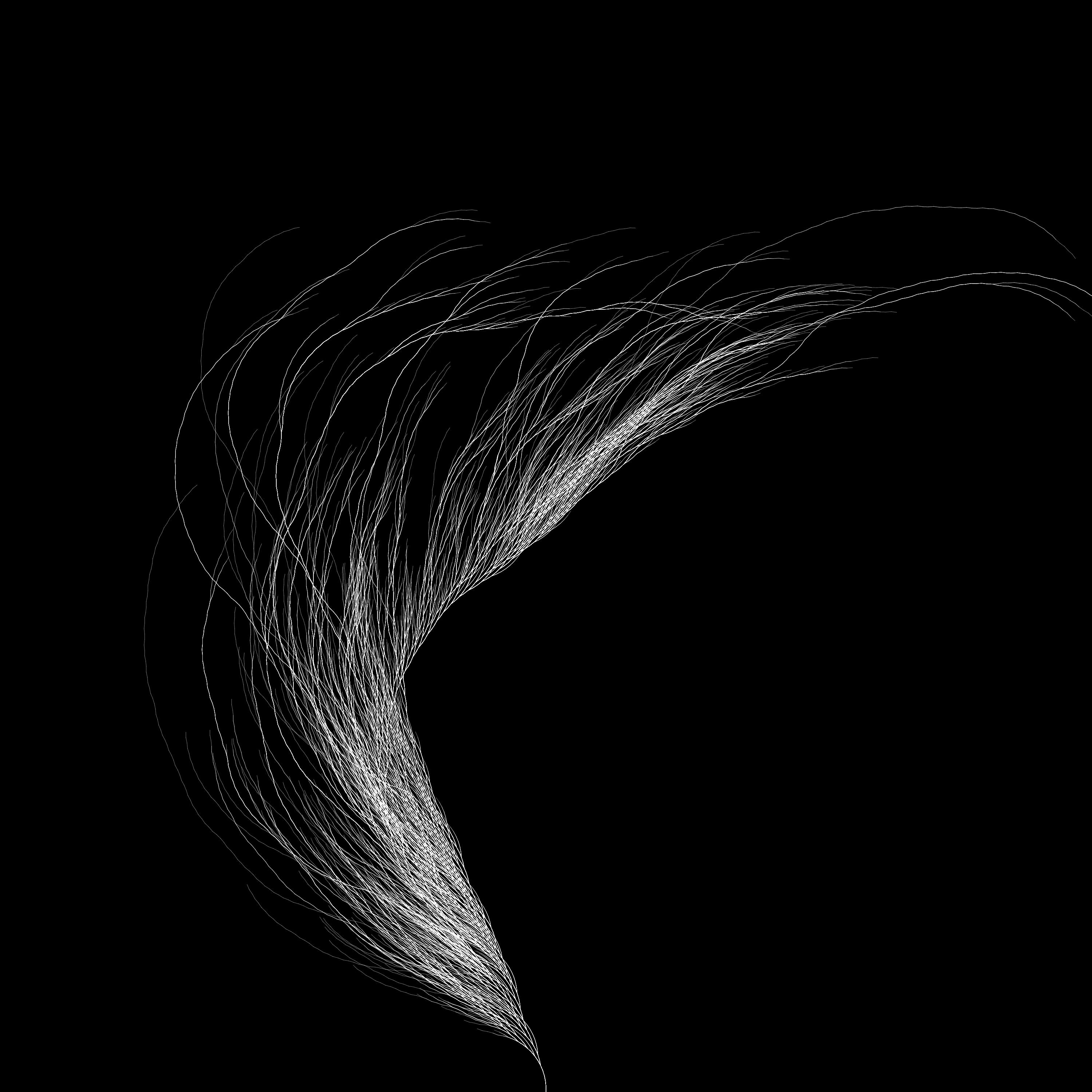
The process is quite simple, for each sequence you generate a line. This line advances a fixed amount for each step of the sequence. If the number if even, we rotate a certain way before advancing, and if the number is odd rotate the other way. If you plot several paths corresponding to several starting numbers on the same image, you get tendrils that I personally think look like coral.
In this particular case, I used p5.js to generate the following figures. The way I did it was starting each sequence from the starting number, then if the number if even rotate clockwise by 0.3 radians, if the number is odd rotate counterclockwise by half that amount.
Using this visualization, by setting the background black, and drawing each path with some transparency, we can see where the sequences overlap. Here is the figure generated for the first 10,000 natural integers.
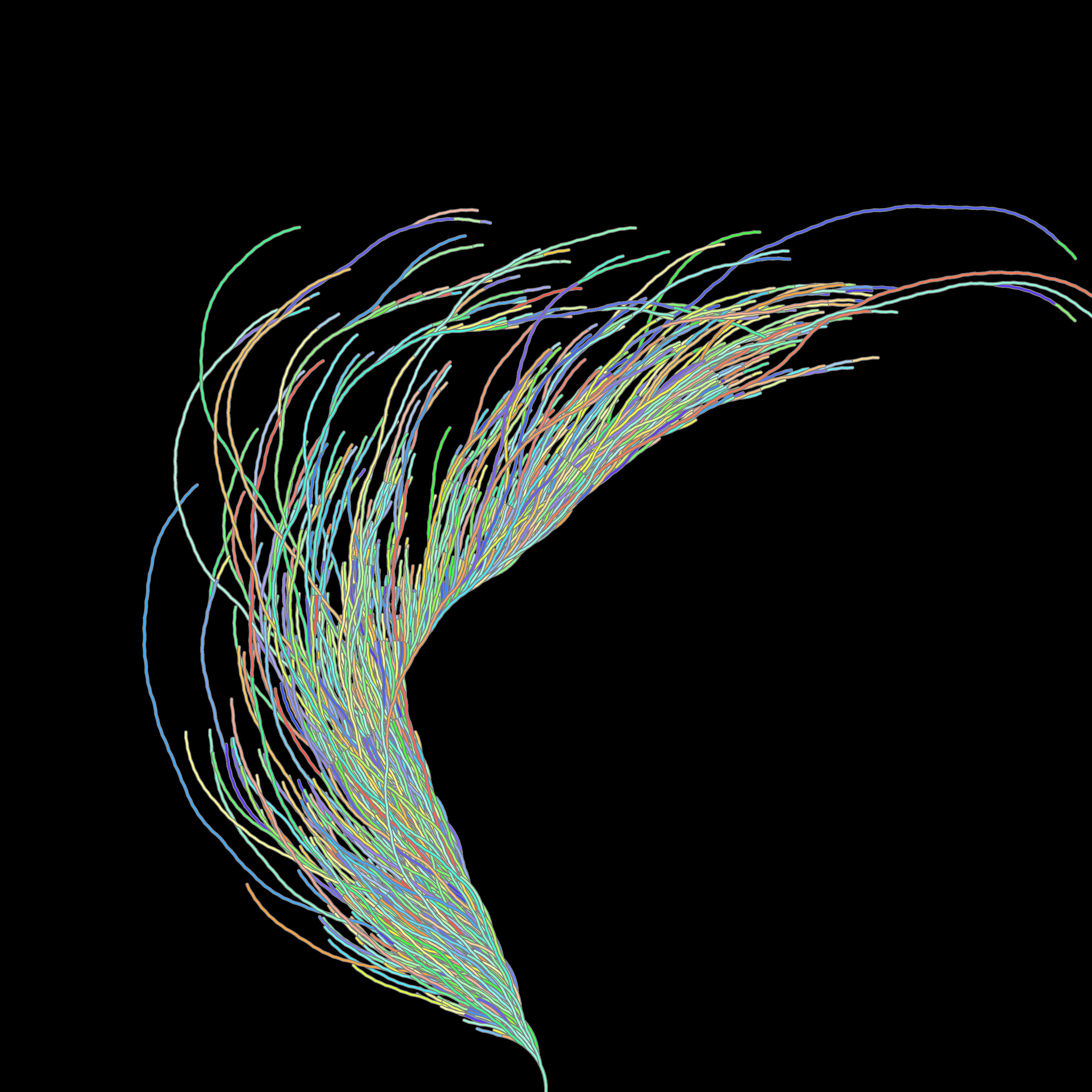
Once we have this basic model it's easy to play a bit. For example here each time I draw a path, I select a random hue and draw the same figure.
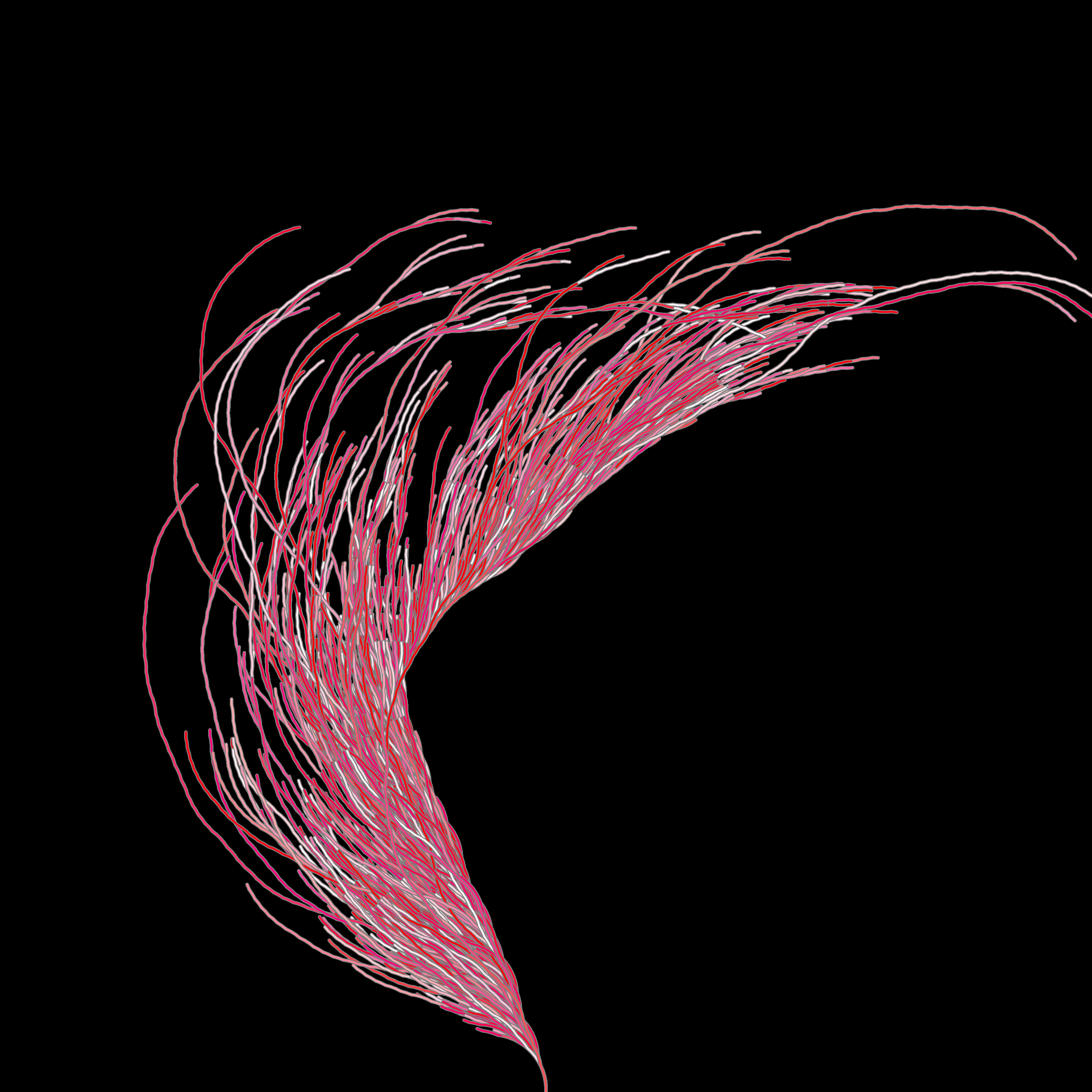
We can restrict the hues to a tighter range, for example only shades of red:
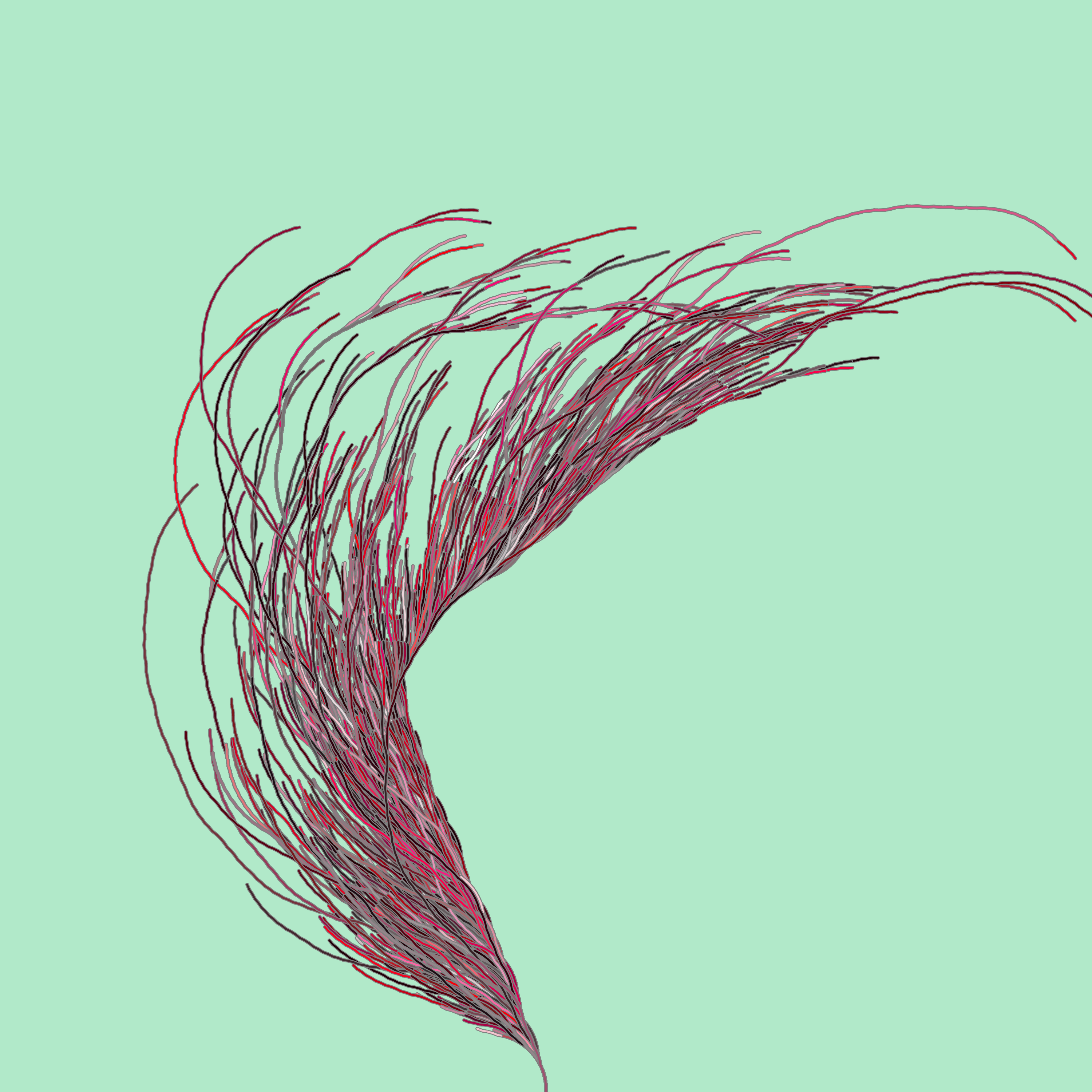
We can also play with the angles a little bit, for example here, for each sequence I draw, I select a random angle between 0.01 and 0.5 radian.
You can also combine that with colors.
Finally I also generated the simple visualization, white paths, for the first 100,000 natural integers. This gives us a much more dense
This skecth is available here if you want to play with it!
Edmund Harris visualization
I was quite happy with these drawings but you migh have noticed they are not really exaclty the same as in the numberphile video. I did a little more digging and realized that there were 2 key differences:
- The collatz sequences used was the "shortcut sequence", where instead of taking \(3\cdot n = 1\) when the number is odd, we take \((3\cdot n + 1)/2\) since we know that \(3\cdot n + 1\) is even.
- Instead of drawing the sequence from the starting number, each line starts with the number 1. And you go backwards in the collatz sequence. If the next number is double the current one, turn clockwise a certain amount, otherwise turn half that amount counter-clockwise.
With these 2 simple changes we can finally get the representation I really wanted for the first 10,000 starting numbers:
Once again, the sketch is availbale here if you want to play with it!
Final thoughts
To be honest I had quite some fun trying to recreate these visualization and I encourage you to do the same. It is however quite hard to come up with original ways of looking at this problem visually. I might come back to it later and update this if I ever do.
In the meantime I hope you enjoyed this article and I'm off to print a large version of that last one for my wall :) !